
When “good enough” has no reward: rethinking cleaning contracts
Improving Cleaning Quality Through Statistical Sampling and Performance Incentives
It is hard to get a consistently high cleaning standard from an external company. The usual problem isn’t the people or the mops — it’s the incentive structure. Do well for months running, and nothing in particular happens: no recognition, no reward. Do badly, and often the same is true: a complaint, a frown, but rarely a consequence that lands where it matters. The only lever most contracts actually pull is binary — pass or fail, renew or don’t — and everything in between goes unmeasured.
Every month we inspect only the number of accommodations or rooms needed for a statistically reliable result. Each inspection produces an objective score. That score determines a monthly bonus or malus for the cleaning company. The result: fewer discussions, better quality, and lower inspection costs.
The rest of this article explains how that works, why it beats a seasonal pass/fail, and where the numbers come from.
The problem
Most cleaning contracts run on two outcomes:
- pass – we continue with you
- fail – we end the contract and will look for another company
There is no incentive for continuous improvement, and no early warning before a full contract review. A team that’s slipping for two months looks identical, on paper, to a team that’s slipping for six — until someone finally notices, usually too late and usually as a dispute.
The solution
Every month:
- Inspect a statistically correct sample — not a fixed percentage. The sample size depends on how many units were cleaned that month.
- Score every defect found, weighted by severity.
- Calculate a single performance score for the month.
- Apply the matching bonus or malus.
Done. No seasonal reviews, no seasonal disputes — feedback and consequence land in the same month the work happened.
| Current system | Proposed system |
|---|---|
| Inspect a fixed 25% | Inspect a statistically correct sample |
| Subjective judgment call | Objective, weighted score |
| Feedback once a season | Feedback every month |
| Pass / fail | Five graduated performance levels |
| Discussions and disputes | Transparent, reproducible scoring |
| Inspection cost scales with a % of all units | Inspection cost scales with statistical need |
Worked example
Park: 320 departures this month.
Sample size (Table C.1, Level II): 50 inspections.
Result: 44 accepted, 6 rejected.
Rejection rate: 12%.
Level: III — exactly meets your chosen threshold derived from the acceptance number, so bonus/malus = 0%.
Had only 3 of the 50 been rejected (6%), the same month would land at Level V (+10% bonus). Had 11 been rejected (22%), it would fall below every defined threshold, defaulting to Level I (−10% malus). Same formula, same sample size, three very different outcomes — and nobody has to argue about which one applies.
Why it works
The sample sizes aren’t arbitrary. They come from BS EN 13549, itself built on ISO 2859 and the older MIL-STD-105E — sampling tables that manufacturing industry has used for inspection since the 1950s. The sample sizes were developed over decades of industrial quality control: they increase with lot size, but much more slowly than a fixed percentage would. That gives a similar level of statistical confidence for both small parks and large ones — something a flat 25% never can, since it under-inspects a small park to the point of meaninglessness and over-inspects a large one at needless expense.
One distinction worth keeping clear: the sampling method — how many units to inspect, and what counts as passing — follows BS EN 13549. The bonus and malus percentages are not part of that standard; they are a management choice, built on top of the measurement system. The standard tells you how confidently how many cleans you have to check and whether you can call a month good or bad; what you do with that verdict is up to you.
The full statistical derivation — sample-size tables, the acceptance-number calculation, and the underlying curves — is in the appendix at the end of this article for anyone who wants to check the work.
The behavioral science
Three findings from behavioral economics explain why this works better than a seasonal pass/fail:
- Monthly feedback changes behavior because people respond much more strongly to immediate consequences than to rewards or penalties that land months later (delay discounting; Ainslie, 1975).
- A modest, reliable malus paired with a generous, frequent bonus steers behavior with less friction than a harsh penalty, because a loss hurts more per euro than an equivalent gain feels good (loss aversion; Kahneman & Tversky, 1979).
- Consequences that scale with severity — five levels instead of pass/fail — outperform all-or-nothing threats, on both the reward and the punishment side (graduated sanctions; Ostrom, 1990).
From individual defect to a single number: demerit scoring
Weighing every defect equally — or worse, stamping a unit simply “clean”/“not clean” — throws away information a well-designed system doesn’t have to throw away. The standard technique is a demerit rating system: assign each defect class a weight, sum the weighted counts into one statistic, and compare it to a threshold.
Translated to a single unit: fatal (wrong or forgotten unit), major (mold, stains, a wet bathroom, leftover food), minor (a few spots, a light layer of dust). Managers immediately see why forgetting an entire room shouldn’t count the same as a dusty shelf.
Scoring rule used in this tool
score = fatal × 9 + major × 3 + minor × 1
Threshold = 9 points — a score above 9 means rejection.
| Class | Weight | Example |
|---|---|---|
| Fatal | 9 | House forgotten / house very badly done |
| Major | 3 | Significant stains or crumbs, floor visibly dirty, leftover food on inventory, clothing left behind |
| Minor | 1 | A few crumbs, light dust, a small stain visible from one angle only |
A single fatal defect already scores 9 on its own, so combined with almost anything else the unit is rejected. A handful of major defects (4 × 3 = 12) or a pile-up of minor ones (10 × 1 = 10) crosses the threshold too — no defect type is capped, each just carries a different weight.
From accepted/rejected houses to bonus or malus
These two tables are how a month’s result turns into money. The method has three steps:
- Count. Take the number of cleans done that month, and look up the matching sample size in table1 in the table section
- Compare. Inspect that sample, count how many were rejected, and check in table 2 that count against the five threshold columns for that row, starting from Level V and working up. The first level whose threshold isn’t exceeded is the month’s level.
- Look up. Take that level to table 3 and read off the matching bonus or malus percentage.
Worked example: 1,000 cleans this month → sample size 80. Say 9 units are rejected. Checking the thresholds for 1,000 cleans (14 / 14 / 10 / 7 / 5): 9 is above the Level V limit (5) and the Level IV limit (7), but at or below the Level III limit (10) — so the month lands on Level III, which the first table shows as 0% bonus/malus. One rejection fewer (8) would still be Level III; three fewer (6) would clear the Level IV threshold and earn a +5% bonus instead.
No discussion, no judgment call — the reject count and the two tables above are the entire decision.
The advantages
- Reproducible. Two different inspectors scoring the same findings land on the same level and the same bonus/malus — no more he-said-she-said over an impression.
- Better-spent inspection hours. Sample size scales with volume, so small sites stop being over-inspected and large ones stop being under-inspected.
- A credible, timely incentive. Monthly, graduated consequences behave the way an incentive is supposed to behave — unlike a threat that only ever shows up as a yes-or-no verdict, months later.
- Less friction, more relationship. A system that mainly rewards invites a cleaning partner to reach for the highest level instead of merely avoiding the lowest.
Tables
Here you can find the tables which are used in this method
Table 1: Sample sizes
Normally level II is used. Level I is for well working cleaning companies. level III is for companies who need more attention
| Lot size (number of cleans) | Level I | Level II | Level III |
|---|---|---|---|
| 2–8 | 2 | 2 | 3 |
| 9–15 | 2 | 3 | 5 |
| 16–25 | 3 | 5 | 8 |
| 26–50 | 5 | 8 | 13 |
| 51–90 | 5 | 13 | 20 |
| 91–150 | 8 | 20 | 32 |
| 151–280 | 13 | 32 | 50 |
| 281–500 | 20 | 50 | 80 |
| 501–1.200 | 32 | 80 | 125 |
| 1.201–3.200 | 50 | 125 | 200 |
| 3.201–10.000 | 80 | 200 | 315 |
| 10.001–35.000 | 125 | 315 | 500 |
| 35.001–150.000 | 200 | 500 | 800 |
| 150.001–500.000 | 315 | 800 | 1250 |
| 500.001+ | 500 | 1250 | 2000 |
Table 2: Calculated thresholds per number of cleans
| Number of cleans | Number of checks | Level I (>) | Level II (≤) | Level III (≤) | Level IV (≤) | Level V (≤) |
|---|---|---|---|---|---|---|
| 50 | 8 | 3 | 3 | 2 | 2 | 1 |
| 100 | 20 | 5 | 5 | 4 | 3 | 2 |
| 200 | 32 | 7 | 7 | 5 | 4 | 3 |
| 500 | 50 | 10 | 10 | 7 | 5 | 3 |
| 1000 | 80 | 14 | 14 | 10 | 7 | 5 |
| 1500 | 125 | 20 | 20 | 14 | 10 | 6 |
| 2000 | 125 | 20 | 20 | 14 | 10 | 6 |
| 3000 | 125 | 20 | 20 | 14 | 10 | 6 |
| 4000 | 200 | 29 | 29 | 21 | 14 | 9 |
| 5000 | 200 | 29 | 29 | 21 | 14 | 9 |
(Level 2, binomial, 98% confidence)
TABLE 3: AQL per level and bonus/malus
| Level I | Level II | Level III | Level IV | Level V | |
|---|---|---|---|---|---|
| AQL | 10% | 10% | 6.5% | 4% | 2% |
| Bonus/malus | −10% | −5% | 0% | +5% | +10% |
📐 Appendix: the statistics behind it, for anyone who wants to check the work
Why the sample sizes grow the way they do
The lot-size boundaries and sample sizes in table 1 were not invented specifically for cleaning — they are almost literally the lot-size code letters and sample sizes from MIL-STD-105E (the American military attribute-sampling standard from the 1950s), carried over into civilian use in ANSI/ASQ Z1.4 and mirrored internationally in ISO 2859-1. BS EN 13549 adopted that generic, decades-proven industry standard for the cleaning sector.
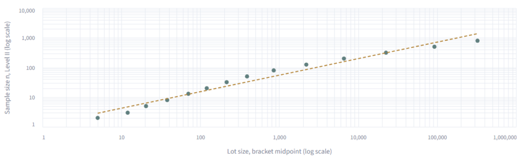
Take the midpoint of each lot-size bracket, take the log of that midpoint and the log of its matching sample size, and plot one against the other: the points fall close to a straight line. A straight line in log-log space means a power law (sample size ∝ lot sizek); fitting that line to Table C.1 gives k ≈ 0.56 (R² ≈ 0.97) — in the same ballpark as, but not exactly, the k=0.5 of a pure square-root law. A fixed percentage is the opposite: sample size = 0.25 × lot size is k=1, a straight line only on a regular (non-log) plot, which is why it produces a different, arbitrary reliability at every lot size.
Why an AQL doesn’t mean you accept that percentage of defects
You never inspect every unit, only a sample — like a blood test, you draw a conclusion about the whole from a small vial, not from testing everything. That’s why the method works with two probabilities instead of one hard cutoff:
- PAQ (Probability of Acceptance at the AQL) — if the true defect rate sits exactly at the AQL threshold, how likely is the sample to still pass it? Deliberately set high (95–98%), to protect the cleaning partner from bad luck in the sample.
- PLQ (Probability of Acceptance at the Limiting Quality) — if the true defect rate is much worse, how likely is the sample to still pass it? Deliberately set low (5–10%).
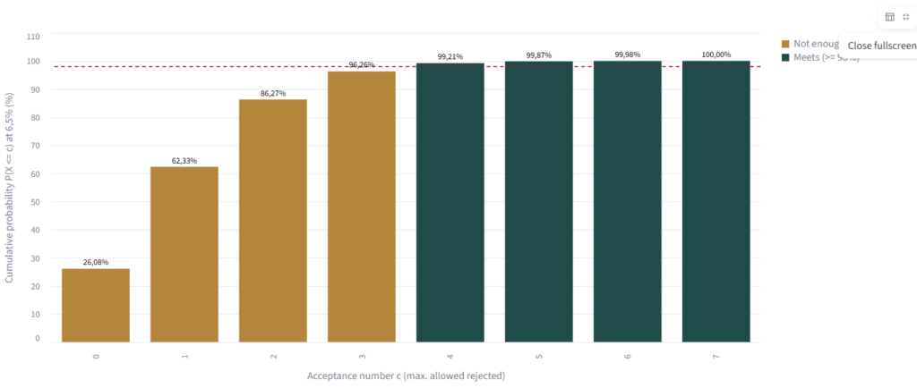
Example: a sample of 20 units, AQL=6.5%, 98% confidence gives acceptance number Ac=4 (PAQ ≈ 99.2%, PLQ at 3×AQL ≈ 65%).
Why do we reject only after 4 rejected houses?
Take AQL = 6.5% on a sample of 20 units. The intuitive reading is to just multiply the two: 6.5% × 20 = 1.3, and conclude that consequences should kick in somewhere around one rejected house. That’s not how the acceptance number works, and the gap between 1.3 and the real threshold of 4 is the whole point.
The 1.3 is only what you’d expect to find if the batch is exactly at the AQL level — it says nothing about certainty. We want to be sure that we reject for a good reason.
Four houses isn’t picked because it “feels” like enough distance from the standard; it’s the smallest cutoff that still lets you say, with 98% confidence, that a batch genuinely performing at 6.5% will pass. Set the bar at 1 or 2 rejects instead, and ordinary sampling luck — which 20 houses happened to get picked that month — would fail plenty of batches that were, in truth, perfectly fine. Four is where that risk drops low enough to trust the verdict.
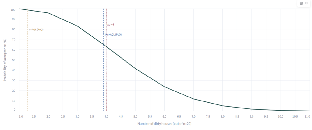
OC curve: probability of acceptance per number of dirty houses
An OC curve (Operating Characteristic curve) shows, for a fixed sample size (20 units) and acceptance number (4), how the probability of accepting a batch changes as the batch’s true defect rate increases. The accept/reject rule itself is a hard cutoff — 4 or fewer rejects in the sample passes, 5 or more fails, always. What the curve shows is something else: because which 20 houses actually get sampled is random, a batch with a given true defect rate won’t always produce the same count of rejects. At low true defect rates, that hard rule accepts almost every time, so the curve sits near 100%. As the true defect rate rises, the same fixed rule starts failing more and more samples, and the curve bends downward toward 0%. The curve isn’t describing a fuzzy pass/fail line — it’s describing how often a fixed, hard rule gets the right answer when applied to random samples from batches of varying true quality.
Discussion: weak points of this method
No method is free of trade-offs, and this one has several worth naming honestly.
The statistics in this method are solid, and the incentive structure is well grounded in established research. That doesn’t make it flawless. Several weaknesses are baked into the design itself, not fixable by tweaking a number, and anyone adopting this should go in with eyes open about them.
1. Accept/reject is still binary — twice over
The headline pitch is “five graduated levels instead of pass/fail.” That’s true at the level of the monthly outcome. But underneath it, two binary decisions are still doing all the work:
- Each inspected unit is judged accept or reject — a demerit score either clears the threshold of 9 or it doesn’t. A unit that scores 8 and a unit that scores 0 are both “accepted”; a unit that scores 10 and a unit that scores 40 are both “rejected.” Real quality differences within each bucket disappear.
- The month is then judged by counting how many of those already-binary units were rejected, and comparing that count to a threshold per level. So the graduation between levels is real, but it’s graduation built entirely on top of a series of yes/no calls, not on a continuous quality signal.
In practice this means two months with very different underlying quality — one full of units scoring 8 (barely acceptable) and one full of units scoring 0 (spotless) — can land on exactly the same level and the same bonus. The method rewards clearing a bar, not how far above it you are.
2. Demerit scoring is subjective, and has to be calibrated
The fatal/major/minor weights (9/3/1) are clean on paper. Applying them in the field is not. “Significant stains,” “a few crumbs,” “visible from one angle” — these all require a human judgment call, and different inspectors will draw the line in different places. A borderline major defect for one inspector might be a minor for another, and that single classification can be the difference between a unit passing or failing.
This is a solvable problem, but it isn’t solved by the scoring rule itself — it requires photo-referenced examples for each severity class, periodic calibration sessions between inspectors, and ideally an inter-rater reliability check (having two inspectors independently score the same units and comparing results) before the numbers are trusted for a bonus/malus decision with real money attached.
3. Small lots get statistically weak samples
The sample-size table is deliberately sub-linear — that’s the whole point of not using a fixed percentage. But at the small end, the absolute sample size is still small: a lot of 20 cleans gets a sample of 5. With that few observations, the confidence the OC curve promises is real in the math, but the practical distance between “this batch is fine” and “this batch is not” is only a couple of rejected units either way. Small locations get a fairer sample size than a flat percentage would give them, but “fairer” doesn’t mean “precise” — the underlying uncertainty of judging quality from 5 inspections is still large.
4. The whole model assumes the sample is actually random
Every probability in this method — PAQ, PLQ, the acceptance number itself — is only valid if the inspected units are a genuinely random draw from that month’s cleans. In practice, sampling is done by a person with a schedule, a map of the park, and limited time. It’s easy, without any bad intent, to end up inspecting whichever units are most convenient, already known to be fine, or flagged by a complaint — and any of those breaks the randomness the statistics depend on. A biased sample doesn’t just add noise; it can make a genuinely bad month look good, or a genuinely good month look bad.
5. The AQL, LQ, and bonus/malus percentages are policy choices, not measurements
It’s easy to read a table with AQL=6.5% and a 98% confidence level and assume those numbers were derived from something — guest complaint data, cost analysis, industry benchmarking. They weren’t. They’re a management choice, same as the bonus and malus percentages next to them. Nothing in BS EN 13549 says 6.5% is the right AQL for a holiday park, or that a Level V month deserves +10% rather than +7% or +15%. That’s not a flaw in the statistics; it’s a reminder that the statistics only tell you how confidently you can measure against a bar you set yourself.
6. A visible formula invites gaming
Once a cleaning company knows exactly how the score is calculated and roughly how sampling works, there’s an incentive to optimize for the measurement rather than for quality itself — extra effort concentrated on units more likely to be sampled, or on the weeks inspections tend to happen, rather than a uniform standard applied every day. This is a general risk with any measurable proxy for a broader goal (sometimes called Goodhart’s law: once a measure becomes a target, it stops being a good measure), and this method doesn’t have a specific defense against it beyond making the sampling schedule genuinely unpredictable.
7. The behavioral-science backing is about individuals, applied to a company
Delay discounting and loss aversion are well-established findings — but they were studied in individual human decision-making, not in how a cleaning company’s management responds to a contractual bonus/malus a step removed from the person actually holding the mop. It’s a reasonable extrapolation, and probably still directionally correct, but it is an extrapolation: nothing here has been tested specifically on cleaning contractors as organizations.
8. A score doesn’t diagnose a root cause
A bad month tells you a bad month happened, at whatever weighted severity the demerit rule computes. It doesn’t tell you why — understaffing, a new hire who wasn’t trained properly, one bad supervisor, high turnover, or just an unlucky sample. The bonus/malus signal is fast and reproducible, but it’s a symptom-level measurement, not a diagnostic one; someone still has to go and find out what actually happened before a malus turns into a fix rather than just a fine.
None of this argues for going back to “we inspect 25%.” A statistically sized sample with a calibrated, transparent scoring rule and a graduated incentive is still a clear improvement over a vague seasonal threat with no defined trigger at all. But it trades one set of problems (arbitrariness, no incentive gradient, no statistical grounding) for a different, smaller set (calibration overhead, sampling discipline, and the honest admission that several of the numbers in the tables are choices, not discoveries). Adopting this method well means managing that second set of problems on purpose, not assuming the math has made them disappear.
Disclaimer
This project is a personal project. It is not endorsed, sponsored, or reviewed by any company I currently work for or have worked for in the past. Those companies have no involvement in it and have no plans to use it.
Sources and further reading
- Shewhart, W.A. (1920s, Bell Telephone Laboratories) — statistical foundation of process control; Dodge, H.F. & Romig, H.G. built practical acceptance-sampling tables on top of it.
- ANSI/ASQ Z1.4, Sampling Procedures and Tables for Inspection by Attributes — civilian successor to MIL-STD-105E; mirrored internationally as ISO 2859-1.
- BS EN 13549:2001, Cleaning services – Basic requirements and recommendations for quality measuring systems, Annex C.
- Ainslie, G. (1975). Specious reward: a behavioral theory of impulsiveness and impulse control. Psychological Bulletin. Generalized by Loewenstein, G. & Prelec, D. (1992), Anomalies in Intertemporal Choice, Quarterly Journal of Economics.
- Kahneman, D. & Tversky, A. (1979). Prospect Theory: An Analysis of Decision under Risk. Econometrica.
- Ostrom, E. (1990). Governing the Commons: The Evolution of Institutions for Collective Action. Cambridge University Press.
- Juran, J.M. — founder of the “cost of quality” framework.
- Journal of Quality Technology, Vol. 31, No. 2 — “Exact Properties of Demerit Control Charts.”
- NEN 2075 / VSR-KMS 3 (Vereniging Schoonmaak Research / Stichting Schoonmaakkwaliteit, 2014); Handboek VSR-Keurmerk, SSK, version 17.01 (2017).
- ISO 22483:2020, Tourism and related services – Hotels – Service requirements.