
From SMA to LOESS
Data Analysis · Climatology · Trend Methods · April 2025
The KNMI uses a LOESS span denominator of 42 to approximate a 30-year running average. But what if you want a different smoothing window? This article derives both the theoretical relationship and an empirical formula — and finds that the two are surprisingly different.
Read also LOESS is more how to use this method easily in Python
1. Background: LOESS and the Running Average
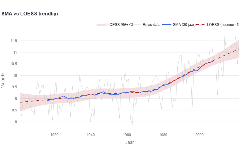
In an earlier post — LOESS is more — I described how the Royal Dutch Meteorological Institute (KNMI) applies the LOESS method as their standard for computing climatological trends. LOESS (Locally Estimated Scatterplot Smoothing) fits local linear regressions to overlapping subsets of the data, rather than imposing a global model.
The KNMI’s choice, documented in Technical Report TR-389 (De Valk, 2020), rests on a key observation: in the centre of a time series, local linear regression with uniform weights over a 30-year window is mathematically identical to the 30-year running average. The LOESS trendline is therefore a well-motivated extension of a method meteorologists have used for decades — one that also provides values at the edges of the record where a centred moving average cannot reach.
The KNMI’s stated reasons for preferring LOESS over a plain moving average are:
- It approximates the classical 30-year climatological running average
- It produces trendline values for the first and last years of the record
- After 21 years, a trendline value is fixed and will not change as new data arrive
- No arbitrary modelling assumptions are required
But the standard LOESS implementation does not use uniform weights — it uses a tricubic weight function. And this changes things. The question becomes: if I want my LOESS curve to match an SMA of x years, what span denominator should I choose?
2. The Theoretical Derivation
Why the window needs to be wider
The tricubic weight function used by standard LOESS is defined as:
f(t) = max{0, 1 − (2|t − t₀| / d)³}³
Unlike a uniform window, this function assigns near-zero weight to observations at the edges of the interval. This means less data effectively contribute to each estimate, which increases the variance of the trendline compared to a uniform-weight average over the same window width. See infobox below for details
To restore variance equality, the window must be widened. The correction factor can be derived from equation (2.44) in Loader (1999), which gives the effective variance of a local polynomial regression estimate as a function of the weight function’s shape. For the tricubic function specifically, TR-389 reports:
Key result (TR-389, Section 2.4): “For the tricubic weight function, a window of 42 years gives the same variance as a 30-year window with uniform weights.”
The general theoretical formula
This gives a simple multiplicative relationship:
LOESS window = SMA window × (42 / 30) ≈ SMA window × 1.417
Theoretical derivation · KNMI TR-389 / Loader (1999) · valid at the centre of the series
The factor 42/30 ≈ 1.417 is the variance-equalising correction for the tricubic kernel. It is not an empirical estimate but a theoretical result derived from the analytical form of the weight function. (see bottom for a derivation)
3. The Empirical Experiment
Method
To test — and possibly refine — this theoretical relationship, I built an interactive Streamlit tool that searches for the best-matching LOESS denominator for each SMA window, using Pearson correlation as the quality criterion. The approach:
- For each SMA window (3–60 years), compute a centred Simple Moving Average
- For each LOESS denominator (10–100), compute the trendline using the exact KNMI parameters
- Find the denominator that maximises Pearson r with the SMA curve
- Fit a linear regression through all (SMA window, best LOESS denominator) pairs
Dataset: annual mean temperatures at De Bilt, 1901–2022 (122 years). The LOESS implementation exactly replicates the KNMI method: degree=1, surface='direct', statistics='exact', iterations=1, via the skmisc.loess library. (see infobox at the bottom)
Result
At first an SMA window of 3-100 was used. This gave a a LOESS-window of 100 after x=60, so the script has been adapted to 3-60.
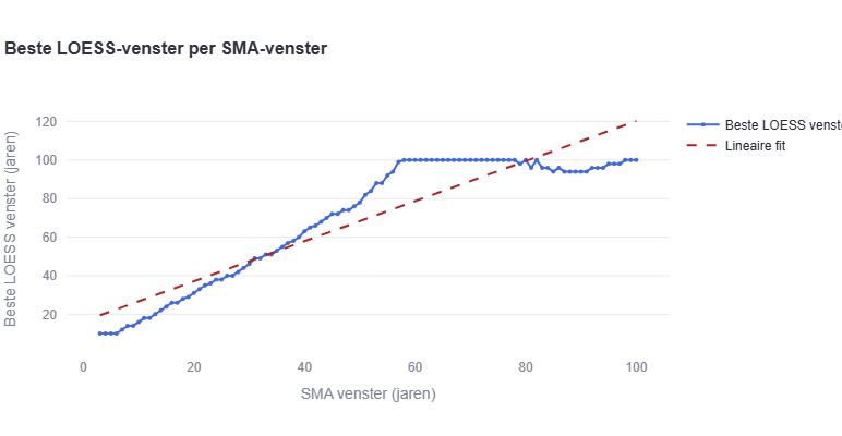
After running the full batch analysis, a remarkably consistent linear relationship emerges:
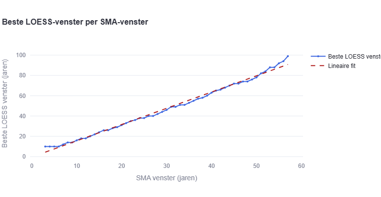
LOESS denominator ≈ 1.618 × SMA window − 1.118
Empirical result · De Bilt 1901–2022 · KNMI LOESS parameters · Pearson r optimisation
The slope of 1.618 is striking: it equals the golden ratio φ. This is almost certainly a coincidence — there is no theoretical reason why the golden ratio should appear here — but it makes the rule of thumb easy to remember. For practical purposes: multiply your SMA window by 1.6 and you have a good starting denominator.
Selected values
| SMA window (years) | Theoretical (×1.417) | Empirical formula | Empirical best |
|---|---|---|---|
| 5 | 7 | 7 | 9 ⚠ |
| 10 | 14 | 15 | 16 |
| 20 | 28 | 31 | 31 |
| 30 | 42 (KNMI) | 47 | 46 |
| 42 | 59 | 67 | 66 |
| 60 | 84 | 96 | 99 |
⚠ At SMA=5, the formula predicts 7 but the empirical optimum is 9. See Section 4.
4. Theory vs. Empirical: Why the Slopes Differ
The theoretical formula predicts a slope of 1.417; the empirical formula finds 1.618. This is a meaningful discrepancy. Several factors explain it:
1. The theoretical result applies only to the centre of the series
The Loader (1999) variance formula holds exactly at the midpoint of the time series, where the LOESS window is fully symmetric. Near the edges of the record, the LOESS algorithm adapts the window shape, changing the effective weight distribution. Pearson correlation integrates the match quality over the entire series — including these edge regions — which inflates the empirically optimal denominator.
2. Variance equality ≠ shape similarity
The theoretical factor equalises variance — the amplitude of fluctuations around the trendline. But Pearson correlation maximises shape similarity: it rewards a curve that rises and falls at the same moments as the SMA, regardless of amplitude. These are related but distinct objectives. A slightly wider LOESS window may track the broader shape of the SMA more faithfully even if its pointwise variance is marginally lower.
3. Small-window edge effects
At SMA=5, the empirical best denominator is 9, but the formula gives 7 — a relative error of about 28%. Small windows are disproportionately affected by edge behaviour because a larger fraction of data points fall near the boundaries. The linear formula is least reliable below SMA ≈ 15.
5. How Much Does It Matter in Practice?
When using the empirical formula rather than the exact optimum, the resulting Pearson r between the LOESS and SMA curves typically remains above 0.99 across the mid-range of window sizes (SMA 15–80 years). The curves are visually indistinguishable. The formula is a reliable starting point; for precision applications, running the correlation optimisation on your specific dataset is recommended.
Practical summary: Use denominator ≈ 1.6 × SMA window as a quick rule of thumb. For the canonical KNMI case (SMA=30), this gives denominator 48 — close to the KNMI’s theoretically derived value of 42. The small difference arises because the KNMI derivation targets variance equality at the series centre, while the empirical optimum minimises the deviation over the full record.
6. Limitations and Further Research
Dataset dependency
The experiment was run on a single time series: 122 years of temperature data from De Bilt. The formula may shift slightly for shorter series, noisier data, different climatological variables, or non-climate contexts. The tool supports uploading your own CSV, so this is easy to verify.
KNMI algorithm parameters
The empirical formula is specific to the exact KNMI parameter set: degree=1, surface='direct', statistics='exact', iterations=1. Changing any of these — for example increasing the degree to 2 (local quadratic regression) — produces a different LOESS curve, and therefore a different optimal denominator per SMA window.
Other data sources
The relationship was derived from temperature data, which is relatively smooth and stationary in variance. For variables with strong heteroscedasticity (e.g. precipitation extremes), the weight function’s behaviour at the edges of the window may matter more, potentially shifting the empirical optimum away from the formula’s prediction.
Open question: the intercept
The formula includes an intercept of −1.118, which is small but non-zero. Theoretically, a denominator of 0 should correspond to an SMA of 0, implying an intercept of exactly 0. The non-zero intercept is an artefact of the discrete search space (denominators start at 10) and the edge effects at small window sizes. It should not be extrapolated below SMA ≈ 5.
Try It Yourself
The tool is available at rcsmit.streamlit.app. You can:
- Upload your own CSV (first column = year/date, second column = value)
- Run the batch analysis to verify the formula for your own time series
- Interactively compare SMA and LOESS and inspect the Pearson r
- View the correlation per LOESS denominator for any chosen SMA window
Conclusion
Two routes lead to the same question — how wide should a LOESS window be to match a given SMA? — and give different answers:
- Theoretical (TR-389 / Loader 1999): multiply by 1.417, based on variance equality for the tricubic kernel at the series centre. This yields the KNMI’s canonical value of 42 for a 30-year SMA.
- Empirical (Pearson optimisation over full series): multiply by 1.618, based on shape-matching over the entire De Bilt record.
The gap between the two — 1.417 vs 1.618 — reflects a genuine difference in what is being optimised: amplitude fidelity at the centre versus shape fidelity across the full record. For most practical uses, the rule denominator ≈ 1.6 × SMA window is a reliable starting point. When precision matters, use the interactive tool to find the optimum for your specific dataset.
So when do you use 1.417, and when 1.618?
| Factor | Use when… | Limitation |
|---|---|---|
| × 1.417 (theoretical) | You want the LOESS trendline to have the same variance as the SMA at the centre of the series — the classical KNMI motivation. | Only exact in the middle of the record. Underestimates the best match near the edges. |
| × 1.618 (empirical) | You want the LOESS curve to look as similar as possible to the SMA across the full length of the series, including the edges. | Derived from one dataset (De Bilt, 122 years). Less reliable for very short series or windows below ~15 years. |
In practice: if your goal is scientific reproducibility of the KNMI standard, use 1.417 (i.e. denominator = 42 for a 30-year SMA). If your goal is visual similarity between the two curves over the whole chart, use 1.618.
References
- De Valk, C.F. (2020). Standard method for determining a climatological trend. KNMI Technical Report TR-389.
- Loader, C. (1999). Local Regression and Likelihood. Springer.
- KNMI. Standaardmethode voor berekening van een trend
- Rene Smit (2024). LOESS is more. rene-smit.com
- Interactive tool: rcsmit.streamlit.app
📊 What is the tricubic weight function?
Say you want to know how warm a typical summer was in 1980. You have data for every year from 1965 to 1995 — 30 years centred on 1980. The question is: how much should each of those years influence your answer?
A plain average says: all years count equally. 1965 counts the same as 1979. LOESS says: that’s not quite right. A year right next to 1980 tells you a lot. A year 15 years away? Much less. So each year gets a weight based on how far it is from the year you’re estimating.
| Year | Distance from 1980 | Weight | Influence |
|---|---|---|---|
| 1980 | 0 | 1.00 | Full |
| 1973 or 1987 | halfway to edge | ~0.6 | Partial |
| 1966 or 1994 | near the edge | ~0.05 | Almost none |
| 1964 or earlier | outside window | 0 | None at all |
The result is a weighted average: multiply each year’s temperature by its weight, add everything up, then divide by the sum of all the weights — not by a flat 30 or 42. Years near zero weight barely move the answer; years with high weight pull it toward themselves strongly.
The “tricubic” part just describes the shape of the taper. The weight drops from 1 at the centre to 0 at the edge following a smooth curve — not a straight line. The double-cubing in the formula makes it flatten out near the centre and fall steeply near the edges.
What happens at the edges of the record?
This is where it gets interesting. When LOESS calculates the value for, say, 1965 — the first year in the De Bilt record — there is no data from 1935 to fill the left half of a symmetric 42-year window. LOESS handles this by shifting the window: instead of centring on 1965, it anchors to the available data and uses 1965–2006 instead. The window is now lopsided — all 42 years sit to the right of the point being estimated.
This has two consequences. First, the weights redistribute: 1965 is no longer at the peak of the curve, so it doesn’t automatically get weight 1.0. Second, the estimate for 1965 leans heavily on years that are further away in time — making it inherently less stable than an estimate in the middle of the record.
This edge behaviour is also why the theoretical correction factor (1.418) and the empirical one (1.618) differ. The theoretical derivation assumes a perfectly symmetric window at every point. The empirical factor was fitted over the full De Bilt record — edges included — and captures the extra instability those lopsided windows introduce.
Why does this create a problem?
Whether in the middle or at the edges, LOESS is always working with less effective data than the nominal window width suggests — because of downweighted edges in the middle, and because of the missing data beyond the record’s endpoints. The fix is to widen the window to 42 years, so that after all that downweighting, the amount of data that actually contributes ends up roughly equal to a plain 30-year average.
Reference: Loader, C. (1999). Local Regression and Likelihood. Springer. Section 2.6.
📐 The Math Behind the 42: Loader’s Derivation
Why does the KNMI use a span denominator of 42 to match a 30-year running average? The answer comes from equalising the variance of two different smoothing methods.
The core idea
A standard 30-year running average weights all years equally — a rectangular window. LOESS uses the tricubic weight function, which gives the centre year full weight and tapers smoothly to zero at the edges. Because the edge years barely contribute, the effective amount of data used is smaller, and the variance of the trendline estimate is therefore higher than for the rectangular window of the same width. To compensate, the window must be widened.
What is variance?
Variance describes how much the estimated trendline would vary if the same method were applied to slightly different data. A lower variance means a more stable and reliable estimate, while a higher variance means the estimate is more sensitive to fluctuations. In smoothing, variance is mainly driven by how much effective data contributes to each estimate.
The variance formula (Loader, 1999, eq. 2.44)
For a weighted local regression, the variance of the trendline estimate at any point is proportional to a variance factor V(W) that depends only on the shape of the weight function:
\[ V(W) = \frac{\int W(v)^2 \, dv}{\left(\int W(v)\, dv\right)^2} \]For a uniform window: the integral of W(v) dv = 2, and the integral of W(v)² dv = 2, so V = 2 / 2² = 0.500.
For the tricubic window: the integral of W(v) dv = 1.157, and the integral of W(v)² dv = 0.949, so V = 0.949 / 1.157² = 0.709.
Setting them equal
Variance is inversely proportional to window width h, so to get the same variance from both methods:
\[ \frac{h_{\mathrm{LOESS}}}{h_{\mathrm{SMA}}} = \frac{V_{\mathrm{tricubic}}}{V_{\mathrm{uniform}}} = \frac{0.709}{0.500} = 1.417 \]Applied to the standard 30-year average: 30 × 1.417 = 42.5 years, which the KNMI rounds down to 42.
Why the empirical formula gives a different slope
The theoretical factor 1.417 is derived for the centre of the time series, where the LOESS window is fully symmetric. Near the edges of the record, LOESS adapts its window shape, which changes the effective weight distribution. The empirical formula in this article — slope 1.618, optimised by Pearson correlation over the full De Bilt record — captures this edge behaviour too. In short: 1.417 = variance equality at the centre; 1.618 = shape similarity across the full series.
Reference: Loader, C. (1999). Local Regression and Likelihood. Springer. Eq. (2.44) and Section 2.6.
⚙️ Why these four LOESS parameters?
The KNMI runs LOESS with four specific settings. Each one is a deliberate choice, not a default.
| Parameter | Value | What it means | Why this choice |
|---|---|---|---|
degree=1 |
linear | For each point, fit a straight line through the nearby years — not a curve. | degree=2 would fit a little parabola that bends to chase local wiggles. A straight local fit gives a smoother, more stable trendline. |
surface='direct' |
exact surface | Calculate the fitted value at every data point exactly, rather than estimating via shortcuts. | The default uses interpolation from a tree structure — fast for millions of points, but imprecise. A climate record has at most a few hundred years, so there is no reason not to do it properly. Also avoids odd behaviour near the edges of the record. |
statistics='exact' |
exact statistics | Compute the uncertainty (standard errors, confidence band) exactly. | The approximate version is a shortcut for large datasets. With a short series, exact computation is fast enough and gives a mathematically correct confidence band around the trendline. |
iterations=1 |
no robustness re-weighting | Do a single pass — do not downweight outliers in extra iterations. | The default (4 iterations) progressively reduces the influence of extreme years so they cannot distort the line. But the KNMI wants extreme years like 2023 to influence the trend — they are real events, not measurement errors. Robustness re-weighting would hide the warming signal. |
In short: these four settings together say “be exact, be simple, and don’t hide the extremes.”


One Comment
Comments are closed.